import numpy as np
import matplotlib.pyplot as plt
from matplotlib.patches import Polygon
from matplotlib.widgets import Slider
from typing import List, Callable
from scipy.optimize import fsolve
# ---- utilities ------------------------------------------
def nest(f: Callable, x, n: int):
for _ in range(n):
x = f(x)
return x
def flatten_once(lst: List[List]):
return [item for sub in lst for item in sub]
# ---- Core fractal logic with varying removal rates --------------------
class TriangleSplitterVarying:
"""
Implements the construction where at iteration j, we remove a triangle
with area ratio r_j relative to the parent triangle.
For the special case r_j = r²/j², the final measure is sin(πr)/(πr).
"""
def __init__(self, r: float, max_iterations: int = 10):
"""
Args:
r: The parameter in r_j = r²/j²
max_iterations: Maximum depth of iteration
"""
self.r = r
self.max_iterations = max_iterations
# Precompute removal ratios
self.removal_ratios = [r**2 / j**2 for j in range(1, max_iterations + 1)]
def compute_split_params(self, removal_ratio: float):
"""
Given a removal ratio r_j, compute the split parameters.
For a triangle with base on bottom, if we remove a triangle from the top
with area ratio r_j, we need to find the height ratio.
Since area scales with height, if we keep a fraction h of the height,
each resulting triangle has area (1-r_j)/2.
The removed triangle has area r_j.
The two remaining triangles together have area (1-r_j).
For symmetric removal from the top, we use:
- center = 0.5 (middle of base)
- The split point determines how much we remove
"""
# For a symmetric split, if we remove area r_j from top,
# the remaining two triangles share area (1-r_j)
# Height ratio of removed triangle: sqrt(r_j)
h_removed = np.sqrt(removal_ratio)
# The split happens at height (1 - h_removed) from bottom
h_split = 1 - h_removed
# For the base of the removed triangle, we need to compute
# the width at height h_split
# For a triangle, width scales linearly with height from apex
# At height h from bottom (where total height is 1),
# the distance from apex is (1-h), so width is proportional to (1-h)
# At the split line, the width ratio is (1 - h_split) = h_removed
# So the split points on the base are at:
# center ± h_removed/2
center = 0.5
half_width = h_removed / 2
left = center - half_width
right = center + half_width
return left, center, right
def split_triangle_at_iteration(self, triangle: np.ndarray, iteration: int):
"""
Split a triangle at a given iteration with removal ratio r_iteration.
"""
if iteration >= len(self.removal_ratios):
return [triangle] # No more splitting
r_j = self.removal_ratios[iteration]
left, center, right = self.compute_split_params(r_j)
a, b, c = triangle
# Points on the base
p_left = b + left * (c - b)
p_right = b + right * (c - b)
# The split happens at these points, creating two triangles
return [
np.array([p_left, b, a]),
np.array([p_right, c, a]),
]
def fractal(self, initial_triangle: np.ndarray, n_iterations: int):
"""
Generate the fractal after n_iterations.
"""
triangles = [initial_triangle]
for iteration in range(min(n_iterations, self.max_iterations)):
new_triangles = []
for tri in triangles:
new_triangles.extend(self.split_triangle_at_iteration(tri, iteration))
triangles = new_triangles
return triangles
# ---- Measure computation ------------------------------------------------
def compute_measure_product(r: float, n_terms: int = 100):
"""
Compute the product: ∏(1 - r²/j²) for j=1 to n_terms
"""
product = 1.0
for j in range(1, n_terms + 1):
product *= (1 - r**2 / j**2)
return product
def compute_measure_sinc(r: float):
"""
Compute sin(πr)/(πr) using the Weierstrass product formula.
"""
if abs(r) < 1e-10:
return 1.0
return np.sin(np.pi * r) / (np.pi * r)
def find_r_for_lambda(target_lambda: float):
"""
Find r such that sin(πr)/(πr) = target_lambda.
"""
def equation(r):
return compute_measure_sinc(r) - target_lambda
# Initial guess
r0 = 0.5
solution = fsolve(equation, r0)
return solution[0]
# ---- Visualization ------------------------------------------------------
def visualize_fractal_with_measure(r: float, max_iterations: int = 8):
"""
Visualize the fractal construction with measure computation.
"""
# Create initial right isosceles triangle with base 2, area 1
# Base from (-1, 0) to (1, 0), apex at (0, 1)
b = np.array([-1.0, 0.0])
c = np.array([1.0, 0.0])
a = np.array([0.0, 1.0])
initial_triangle = np.array([a, b, c])
fig, axes = plt.subplots(2, 4, figsize=(16, 8))
axes = axes.flatten()
splitter = TriangleSplitterVarying(r, max_iterations)
# Compute theoretical measure
measure_theory = compute_measure_sinc(r)
measure_product = compute_measure_product(r, max_iterations)
fig.suptitle(
f'Fractal Construction with r = {r:.4f}\n'
f'Theoretical Measure λ = sin(πr)/(πr) = {measure_theory:.6f}\n'
f'Product Formula (n={max_iterations}): {measure_product:.6f}',
fontsize=12, fontweight='bold'
)
for idx, n in enumerate(range(9)):
if idx >= len(axes):
break
ax = axes[idx]
triangles = splitter.fractal(initial_triangle, n)
# Compute actual measure (sum of triangle areas)
total_area = sum(triangle_area(tri) for tri in triangles)
for tri in triangles:
ax.add_patch(
Polygon(
tri,
closed=True,
edgecolor='black',
facecolor='lightblue',
linewidth=0.5,
)
)
ax.set_xlim(-1.2, 1.2)
ax.set_ylim(-0.1, 1.2)
ax.set_aspect('equal')
ax.set_title(f'Iteration {n}\nArea = {total_area:.6f}', fontsize=10)
ax.grid(True, alpha=0.3)
plt.tight_layout()
return fig
def triangle_area(triangle: np.ndarray):
"""
Compute the area of a triangle using the cross product formula.
"""
a, b, c = triangle
return 0.5 * abs(np.cross(b - a, c - a))
# ---- Interactive visualization with slider ------------------------------
def interactive_measure_exploration():
"""
Interactive exploration of the relationship between r and measure λ.
"""
fig = plt.figure(figsize=(14, 10))
# Create subplots
ax_fractal = plt.subplot(2, 2, (1, 3))
ax_graph = plt.subplot(2, 2, 2)
ax_product = plt.subplot(2, 2, 4)
plt.subplots_adjust(bottom=0.15, hspace=0.3)
# Initial parameters
r0 = 0.5
max_iter = 8
# Create initial triangle
b = np.array([-1.0, 0.0])
c = np.array([1.0, 0.0])
a = np.array([0.0, 1.0])
initial_triangle = np.array([a, b, c])
def redraw(r, n_iter):
# Clear axes
ax_fractal.clear()
ax_graph.clear()
ax_product.clear()
# Generate fractal
splitter = TriangleSplitterVarying(r, max_iter)
triangles = splitter.fractal(initial_triangle, n_iter)
# Draw fractal
for tri in triangles:
ax_fractal.add_patch(
Polygon(
tri,
closed=True,
edgecolor='black',
facecolor='lightblue',
linewidth=0.5,
)
)
total_area = sum(triangle_area(tri) for tri in triangles)
measure_theory = compute_measure_sinc(r)
ax_fractal.set_xlim(-1.2, 1.2)
ax_fractal.set_ylim(-0.1, 1.2)
ax_fractal.set_aspect('equal')
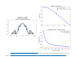
ax_fractal.set_title(
f'Iteration {n_iter}, r = {r:.4f}\n'
f'Actual Area: {total_area:.6f}\n'
f'Theory λ = sin(πr)/(πr): {measure_theory:.6f}',
fontsize=11
)
ax_fractal.grid(True, alpha=0.3)
# Plot measure vs r
r_values = np.linspace(0.01, 0.99, 200)
lambda_values = [compute_measure_sinc(r_val) for r_val in r_values]
ax_graph.plot(r_values, lambda_values, 'b-', linewidth=2, label='λ = sin(πr)/(πr)')
ax_graph.plot(r, measure_theory, 'ro', markersize=10, label=f'Current: r={r:.3f}, λ={measure_theory:.3f}')
ax_graph.set_xlabel('r', fontsize=11)
ax_graph.set_ylabel('λ (Measure)', fontsize=11)
ax_graph.set_title('Measure vs Parameter r', fontsize=11)
ax_graph.grid(True, alpha=0.3)
ax_graph.legend()
ax_graph.set_xlim(0, 1)
ax_graph.set_ylim(0, 1)
# Plot convergence of product
iterations = range(1, 21)
product_values = [compute_measure_product(r, n) for n in iterations]
ax_product.plot(iterations, product_values, 'b-o', linewidth=2, markersize=4, label='Product formula')
ax_product.axhline(y=measure_theory, color='r', linestyle='--', linewidth=2, label='Theoretical limit')
ax_product.set_xlabel('Number of terms', fontsize=11)
ax_product.set_ylabel('Product value', fontsize=11)
ax_product.set_title(f'Convergence of ∏(1 - r²/j²) for r={r:.4f}', fontsize=11)
ax_product.grid(True, alpha=0.3)
ax_product.legend()
fig.canvas.draw_idle()
# Create sliders
ax_r = plt.axes([0.15, 0.05, 0.7, 0.03])
ax_iter = plt.axes([0.15, 0.01, 0.7, 0.03])
s_r = Slider(ax_r, 'r', 0.01, 0.99, valinit=r0)
s_iter = Slider(ax_iter, 'iterations', 0, max_iter, valinit=max_iter, valstep=1)
def update(_):
redraw(s_r.val, int(s_iter.val))
s_r.on_changed(update)
s_iter.on_changed(update)
redraw(r0, max_iter)
plt.show()
# ---- Examples for specific target measures -----------------------------
def show_specific_measures():
"""
Show fractals with specific target measures.
"""
target_lambdas = [0.9, 0.7, 0.5, 0.3]
fig, axes = plt.subplots(2, 2, figsize=(12, 12))
axes = axes.flatten()
b = np.array([-1.0, 0.0])
c = np.array([1.0, 0.0])
a = np.array([0.0, 1.0])
initial_triangle = np.array([a, b, c])
for idx, target_lambda in enumerate(target_lambdas):
ax = axes[idx]
# Find r for this lambda
r = find_r_for_lambda(target_lambda)
# Generate fractal
splitter = TriangleSplitterVarying(r, max_iterations=10)
triangles = splitter.fractal(initial_triangle, 10)
# Draw
for tri in triangles:
ax.add_patch(
Polygon(
tri,
closed=True,
edgecolor='black',
facecolor='lightblue',
linewidth=0.3,
)
)
total_area = sum(triangle_area(tri) for tri in triangles)
ax.set_xlim(-1.2, 1.2)
ax.set_ylim(-0.1, 1.2)
ax.set_aspect('equal')
ax.set_title(
f'Target λ = {target_lambda:.1f}\n'
f'r = {r:.4f}\n'
f'Actual area = {total_area:.4f}',
fontsize=11
)
ax.grid(True, alpha=0.3)
fig.suptitle(
'Fractal Sets with Prescribed Measures\n'
'Using r_j = r²/j² and λ = sin(πr)/(πr)',
fontsize=13, fontweight='bold'
)
plt.tight_layout()
return fig
# ---- Main ----------------------------------------------------------------
if __name__ == "__main__":
print("Fractal Construction with Prescribed Measure")
print("=" * 60)
print("\nTheory: For r_j = r²/j², the limiting measure is:")
print("λ = sin(πr)/(πr)")
print("\nThis allows constructing a set with ANY measure λ ∈ (0,1)")
print("by choosing appropriate r ∈ (0,1)")
print("=" * 60)
# Example calculations
print("\nExamples:")
for target_lambda in [0.9, 0.7, 0.5, 0.3, 0.1]:
r = find_r_for_lambda(target_lambda)
actual_lambda = compute_measure_sinc(r)
print(f" Target λ = {target_lambda:.1f} → r = {r:.6f} → λ = {actual_lambda:.6f}")
print("\n" + "=" * 60)
print("Generating visualizations...")
print("=" * 60)
# Generate static visualizations
fig1 = visualize_fractal_with_measure(r=0.5, max_iterations=8)
fig1.savefig('fractal_iterations.png', dpi=150, bbox_inches='tight')
print("✓ Saved: fractal_iterations.png")
fig2 = show_specific_measures()
fig2.savefig('fractal_specific_measures.png', dpi=150, bbox_inches='tight')
print("✓ Saved: fractal_specific_measures.png")
# Launch interactive visualization
print("\nLaunching interactive visualization...")
print("Use sliders to explore different values of r and iterations")
interactive_measure_exploration()